Movies

library(tidyverse)
library(here)
library(lubridate)
library(MetBrewer) #Met Palette Generator
library(ggplot2)
library(hrbrthemes)
library("viridis")           
library(scales)
library(ggstream)
library(cowplot)

na_strings <- c("$", ",")

movies <- read_delim("data/movies.csv", delim = ";", 
                     escape_double = FALSE, trim_ws = TRUE, 
                     skip = 1) %>% 
  select(Rank, Title, Gross =  `Lifetime Gross`, Year) %>% 
  mutate(Gross_num = as.numeric(gsub("[[:punct:]]", "", Gross)),
         Title = replace(Title, is.na(Gross_num), "")) %>% 
  mutate(Gross_num = replace(Gross_num, is.na(Gross_num), 0)) 
         
Year <- sort(unique(movies$Year))
Year_all <- 1997:2021
Year_missing <- setdiff(Year_all, Year)
Year_missing

add_tibble <- tibble(
  Rank = rep(NA, length(Year_missing)), 
  Title = as.character(1:length(Year_missing)),
  Year = Year_missing, 
  Gross_num = rep(-4000000000, length(Year_missing))
)


movies2 <- bind_rows(movies, add_tibble) %>% 
  mutate(Title = fct_reorder(Title, Year)) 


my_color <- c("#ffffff", rep("#231f20", 11), 
              "#ffffff", "#231f20", 
              rep("#ffffff", 4), "#231f20", 
              rep("#ffffff", 4), "#231f20", 
              rep("#ffffff", 10), "#231f20", "#ffffff")

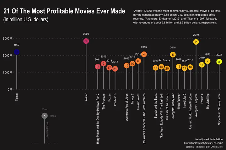
p_title <- "21 Of The Most Profitable Movies Ever Made"
p_subtitle <- "(in million U.S. dollars)\n"


# lollipop chart
p <- ggplot(movies2, aes(Gross_num, Title)) +
  geom_segment(aes(x = 0, y = Title, xend = Gross_num, yend = Title), 
               color = "grey50",
               size = 0.85) +
  geom_point(aes(color = as.character(Year)), size = 6) +
  geom_text(aes(label = Rank), color = "#231f20", size = 2.75) +
  geom_text(aes(label = Year), 
            color = "white", 
            size = 2.25,
            hjust = 0.5,
            vjust = -3.5) +
  coord_flip() +
  scale_color_viridis(discrete = TRUE, option = "C")+
  scale_fill_viridis(discrete = TRUE) +
  scale_x_continuous(labels = unit_format(unit = "M", scale = 1e-6),
                     limits = c(0, 3500000000)
                     ) +
  labs(title = p_title,
       subtitle = p_subtitle) +
  theme_ipsum() +
  theme(
    plot.background = element_rect(fill="#231f20", 
                                   color="#231f20"),
    plot.margin = margin(0.75, 0.3, 0.5, 0.25, "cm"),
    plot.title = element_text(size = 18,
                              hjust = -0.11,
                              face = "bold",
                              color="#ffffff"),
    plot.subtitle = element_text(size = 14,
                                 hjust = -0.06,
                                 color="#ffffff"),
    legend.position = "none",
    panel.grid.major.y = element_line(
      size = .1,
      linetype = 3
    ),
    panel.grid.major.x = element_blank(),
    panel.grid.minor = element_blank(),
    axis.title.x = element_blank(),
    axis.title.y = element_blank(),
    axis.text.x = element_text(size = 8,
                               hjust = 1,
                               vjust = 0.5,
                               angle = 90,
                               color=my_color),
      axis.text.y = element_text(size = 8,
                                 color="#ffffff")) 
  
p  

p2 <- ggplot() +
  geom_segment(aes(x = 0, xend = 0, 
                   y = 0, yend = 5),
               size = 0.85,
               colour = "grey50") +
  geom_point(aes(x=0, y = 5), 
             size = 6,
             colour = "grey50",
             stroke = 1) +
  geom_text(aes(x = 0, y = 5, label = "X"),
            colour = "white",
            hjust = 0.5,
            vjust = 0.5,
            size = 2.75) +
  geom_text(aes(x = 0, y = 6.2, label = "Year"),
            color = "grey50", 
            size = 2.25,
            hjust = 0.5) +
  geom_text(aes(x = 0.33, y = 5, label = "Rank"),
            color = "grey50", 
            size = 2.25,
            hjust = 0.5) +
  geom_text(aes(x = 0.1, y = 2.4, label = "Lifetime Gross"),
            color = "grey50", 
            size = 2.25,
            hjust = 0.5,
            angle = 90) +
  scale_y_continuous(limits = c(0, 6.5), breaks = seq(0, 7, 7)) +
  scale_x_continuous(limits = c(-0.5, 0.5))+
  theme_minimal() +
  theme(plot.background = element_rect(fill="#231f20", 
                                       color="#231f20"),
        panel.grid.major.y = element_line(
          size = .1,
          linetype = 3,
          color = "grey50"),
        axis.text = element_blank(),
        axis.title = element_blank(),
        panel.grid = element_blank())

p2   

ggdraw(p) +
  draw_plot(p2, 
            hjust = -0.5, 
            vjust = .1, 
            width = 0.195, 
            height= 0.4, 
            scale = 0.75) +
draw_text(text= '"Avatar" (2009) was the most commercially successful movie of all time, \nhaving generated nearly 2.85 billion U.S. dollars in global box office \nrevenue. "Avengers: Endgame" (2019) and "Titanic" (1997) followed,\nwith revenues of about 2.8 billion and 2.2 billion dollars, respectively.', 
          x=0.59,
          y=0.8891, 
          size=7, 
          hjust = 0,
          color="#ffffff")  +
  draw_text(text= "Not adjusted for inflation", 
            x=0.985, 
            y=0.072, 
            size=6, 
            hjust = 1,
            color="#ffffff",
            fontface="bold")  +
  draw_text(text= "Estimated throught January 18, 2022", 
            x=0.985, 
            y=0.047, 
            size=6, 
            hjust = 1,
            color="#ffffff",
            fontface="italic")  +
  draw_text(text = "@leynu_ | Source: Box Office Mojo", 
            x=0.985, 
            y=0.022, 
            color="#ffffff", 
            size=6, 
            hjust = 1)

ggsave("~/Desktop/movies.png",
       width=2400/300, 
       height =1600/300)